Analysis of Stereo-seq mouse olfactory bulb dataset#
In this tutorial, we demonstrate SpaRCL on the analysis of Stereo-seq mouse olfactory bulb dataset including
Spatial reconstruction
Mini-batch relational contrastive learning
Spatial domain identification
Finding differentially expressed genes
Spatial domain annotation
The dataset is available at JinmiaoChenLab GitHub (data >> Stero-seq.tar.gz).
[1]:
import numpy as np
import pandas as pd
import scanpy as sc
import matplotlib.pyplot as plt
import seaborn as sns

import SpaRCL as rcl
Data loading and preprocessing#
We load the dataset and find top 8000 highly variable genes.
[2]:
adata = sc.read_h5ad('./data/Stereo_seq.h5ad')
adata
[2]:
AnnData object with n_obs × n_vars = 19527 × 27106
    obsm: 'spatial'
[3]:
sc.pp.highly_variable_genes(adata, n_top_genes=8000, flavor='seurat_v3')
Spatial reconstruction#
We perform spatial reconstruction to aggregate expression from spatial neighbors.
[4]:
rcl.spatial_reconstruction(adata, n_neighbors=30)
Mini-batch relational contrastive learning#
We select 4000 reference centers and then perform mini-batch relational contrastive learning on the reconstructed data.
[5]:
sc.pp.pca(adata)
rcl.reference_centers(adata, n_centers=4000)
C:\ProgramData\Anaconda3\lib\site-packages\sklearn\cluster\_kmeans.py:887: UserWarning: MiniBatchKMeans is known to have a memory leak on Windows with MKL, when there are less chunks than available threads. You can prevent it by setting batch_size >= 4096 or by setting the environment variable OMP_NUM_THREADS=1
  warnings.warn(
Since this step takes some time, we load previously computed AnnData.
[6]:
# rcl.run_RCL_minibatch(adata)

adata = sc.read_h5ad('./data/Stereo_seq_results.h5ad')
adata
[6]:
AnnData object with n_obs × n_vars = 19527 × 27106
    obs: 'reference_centers'
    var: 'highly_variable', 'highly_variable_rank', 'means', 'variances', 'variances_norm'
    uns: 'hvg', 'relation', 'pca', 'reference_centers', 'spatial_reconstruction'
    obsm: 'X_pca', 'relation', 'spatial'
    varm: 'PCs'
    layers: 'counts', 'log1p'
Spatial domain identification#
We create a temporary AnnData using the sample-by-reference relation matrix and then interoperate with SCANPY to identify spatial domains.
[7]:
adata_V = sc.AnnData(adata.obsm['relation'])
adata_V.obs_names = adata.obs_names
adata_V.obsm['spatial'] = adata.obsm['spatial']
adata_V
[7]:
AnnData object with n_obs × n_vars = 19527 × 3983
    obsm: 'spatial'
[8]:
sc.pp.pca(adata_V)
sc.pp.neighbors(adata_V)
[9]:
sc.tl.louvain(adata_V, resolution=0.4)
[10]:
adata.obs['louvain'] = adata_V.obs['louvain']
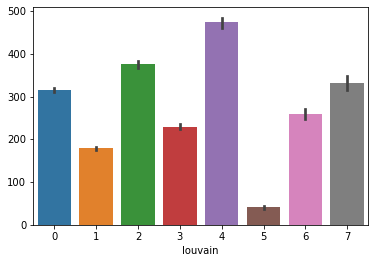
We exclude domain 5 from downstream analysis, since its average count is lower than 100.
[11]:
sns.barplot(y=np.sum(adata.layers['counts'].toarray(), axis=1), x=adata.obs['louvain'])
[11]:
<AxesSubplot:xlabel='louvain'>
[12]:
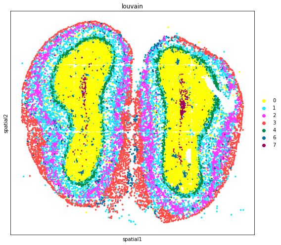
adata_subset = adata[~adata.obs['louvain'].isin(['5']),:]
[13]:
fig, axs = plt.subplots(figsize=(8, 7))

sc.pl.embedding(
    adata_subset,
    basis='spatial',
    color='louvain',
    size=50,
    palette=sc.pl.palettes.default_102,
    legend_loc='right margin',
    show=False,
    ax=axs,
)

plt.tight_layout()
Trying to set attribute `.uns` of view, copying.
Finding differentially expressed genes#
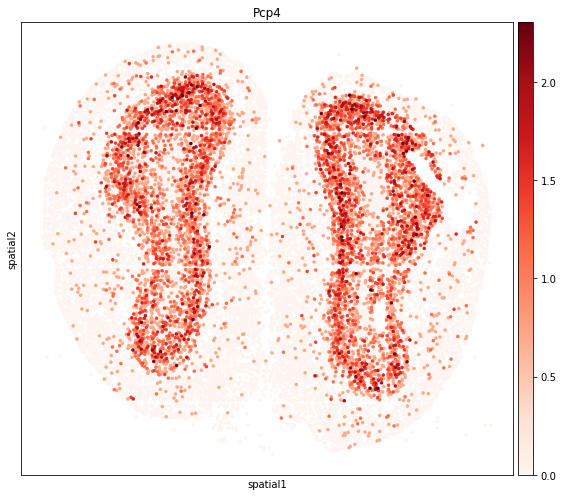
We find the differentially expressed (DE) genes across identified domains and show the domains and their DE gene expression patterns in spatial coordinates.
[14]:
sc.tl.rank_genes_groups(adata_subset, groupby='louvain', use_raw=False, layer='counts', method='t-test_overestim_var')
[15]:
de_genes = pd.DataFrame(adata_subset.uns['rank_genes_groups']['names']).iloc[:10,:]
de_genes
[15]:
| 0 | 1 | 2 | 3 | 4 | 6 | 7 | |
|---|---|---|---|---|---|---|---|
| 0 | Pcp4 | Vip | Cmss1 | Apod | Nme7 | Hbb-bs | Plp1 |
| 1 | Nrxn3 | Lcat | Gm42418 | Ptn | Snap25 | Hba-a1 | Mbp |
| 2 | Ppp3ca | Fam98c | Cck | Ptgds | Scg2 | Hbb-bt | Fth1 |
| 3 | Kcnb2 | Gm10610 | Cdk8 | Atp1a2 | Gabra1 | Hba-a2 | Trf |
| 4 | Camk2n1 | Ly6c1 | Nrsn1 | Apoe | Gm42418 | Ptgds | Cldn11 |
| 5 | Tshz1 | Gm48843 | Calb2 | Fabp7 | Cpe | Apex2 | Mal |
| 6 | Meis2 | Vmn1r67 | Nxph1 | S100a5 | Uchl1 | Mgp | Sox11 |
| 7 | Pbx3 | Esp34 | Olfm1 | Kctd12 | Syt1 | Igf2 | Mag |
| 8 | Camk2b | Tnfsf15 | Sparcl1 | Gng13 | Cltc | Dcn | Zfp704 |
| 9 | Calm2 | AC124606.2 | Ptprd | Npy | Slc17a7 | Acta2 | Mobp |
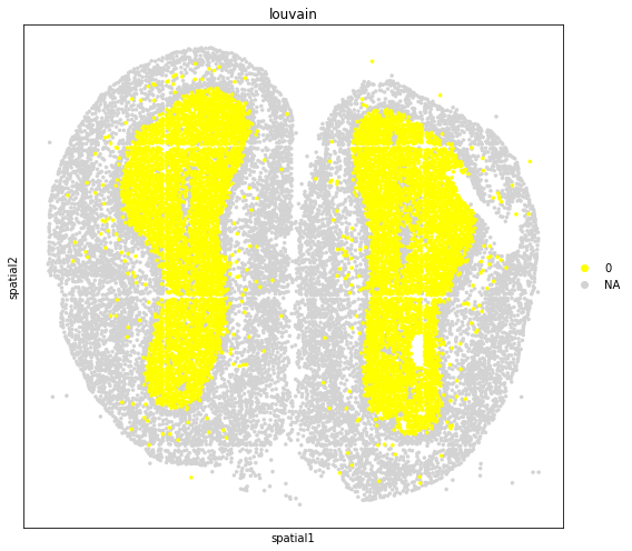
[16]:
fig, axs = plt.subplots(figsize=(8, 7))

sc.pl.embedding(
    adata_subset,
    basis='spatial',
    color='louvain',
    groups='0',
    layer='log1p',
    size=50,
    palette=sc.pl.palettes.default_102,
    legend_loc='right margin',
    show=False,
    ax=axs,
)

plt.tight_layout()
[17]:
fig, axs = plt.subplots(figsize=(8, 7))

sc.pl.embedding(
    adata_subset,
    basis='spatial',
    color=de_genes.iloc[0,0],
    layer='log1p',
    size=50,
    color_map='Reds',
    vmax='p99.9',
    show=False,
    ax=axs,
)

plt.tight_layout()
[18]:
fig, axs = plt.subplots(figsize=(8, 7))

sc.pl.embedding(
    adata_subset,
    basis='spatial',
    color='louvain',
    groups='3',
    layer='log1p',
    size=50,
    palette=sc.pl.palettes.default_102,
    legend_loc='right margin',
    show=False,
    ax=axs,
)

plt.tight_layout()

[19]:
fig, axs = plt.subplots(figsize=(8, 7))

sc.pl.embedding(
    adata_subset,
    basis='spatial',
    color=de_genes.iloc[0,3],
    layer='log1p',
    size=50,
    color_map='Reds',
    vmax='p99.9',
    show=False,
    ax=axs,
)

plt.tight_layout()

Spatial domain annotation#
We annotate the spatial domains based on the anatomical annotation from Fu, H. et al. and marker genes.
[20]:
map_dict = {
    '0': 'GCL',
    '1': 'EPL',
    '2': 'GL',
    '3': 'ONL',
    '4': 'MCL',
    '6': 'BLD',
    '7': 'RMS',
}
[21]:
adata_subset.obs['annotation'] = adata_subset.obs['louvain'].map(map_dict).astype('category')
[22]:
fig, axs = plt.subplots(figsize=(8.3, 7))

sc.pl.embedding(
    adata_subset,
    basis='spatial',
    color='annotation',
    size=50,
    palette=sc.pl.palettes.default_102,
    legend_loc='right margin',
    show=False,
    ax=axs,
)

plt.tight_layout()
